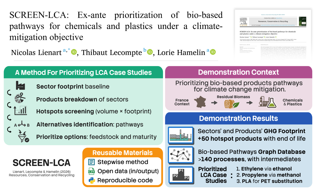
We have recently published “SCREEN-LCA”, a method which we developed and tested during my PhD. As the name suggests, it is a screening method to help prioritize LCA case studies. More specifically, we made it to select the most promising substitutes to high-environmental-footprint products in a given product sector. Indeed, selection is unavoidable when facing many possibilities such as in the bio-based sector.

In this post, I go beyond the article’s specific scope and share about some additional takeaways, which could be useful for the community.

Article:
Lienart, Nicolas, Lecompte, Thibaut, & Hamelin, Lorie (2027).
SCREEN-LCA: Ex-ante prioritization of bio-based pathways for chemicals and plastics under a climate-mitigation objective.
Resources, Conservation and Recycling, 237, 109198.
https://doi.org/10.1016/j.resconrec.2026.109198

Table of content

A bit of context

Skip if you already know about LCA and the challenges associated with finding “good” case studies.

This work originates from our difficulties when navigating in realm of bio-based products. My PhD research considers agriculture residues as a resource for the bioeconomy (e.g., straw, food waste, forestry residues, etc.). We want to identify the most environmentally favourable pathways, starting from residues and producing chemicals and materials, we are especially interested in the climate change mitigation potential. Life cycle assessment (LCA) is our favourite method to estimate environmental footprints. Yet, anyone who has ever conducted an LCA knows how much time- and data-intensive it can be. Good data needs to be found, organized, implemented in a model and to make sense of the results. It would be hopeless, considering our limited time, to produce as many good LCA as there are bio-based products and ways to obtain them. Just imagine all possible things which we call “chemicals”, “materials” or “products” surrounding us.

Yet, it didn’t take us long before we crossed the road of some famous bio-based chemicals and materials. Everyone in the field talk about polylactic acid (PLA), polyhydroxyalkanoates (PHAs), succinic acid, ethanol, glycerol or “hempcrete” (hemp-based concrete), to name a few. So, why not simply consider them as our LCA case studies if they are so prominent?

It was not a good justification, for us, to restrain our investigation to these on the sole ground of trend. What purpose do they have? Which products are they intended to replace? We are convinced that climate change mitigation cannot be addressed without raising the question of replacing (or altogether stopping) some problematic products. It goes beyond taking any bio-based products as inherently sustainable.

As we were lacking a clear picture of the bio-based products we need, and no reusable and consistent method was available in the literature to help us prioritize our LCA efforts, we set out to address the question ourselves.

Goal of the method

Skip if you already know what the article is about.

Based on the principle that we can’t conduct as many full-fledged LCA studies as there are possible bio-based pathways, we thought of making a case study selection method coherently with our objective. SCREEN-LCA is here to fill this gap. Through this method, we can restrain the spectrum of options to just a handful of promising case studies. These must hold a high potential in terms of environmental impact mitigation, technical and economical short-term feasibility. Then, drawing from this selection, we can move to the bottleneck but important step of properly estimating the potential via LCA.

We didn’t start from a bio-based alternative entry point but instead took the perspective of current environmental hotspots. SCREEN-LCA works like this:

1. We confirm that the sectors we want to address (e.g., chemicals) have large impacts (according to the chosen indicator) within the region of interest (could be multiple). For example, we are interested in the French chemical industry. Yet, is it even a large contributor to our climate change indicator nowadays considering outsourcing of production? Also, we look at production and import flows at the same time, with the rationale that the region of interest regulates these internal flows.
2. We identify the “hotspot” products within the sector (breakdown): We start by selecting the most voluminous flows, these are then screened based on their footprints by using the same indicator as in the previous step. Note that footprint data is generally more difficult to obtain than volumes, hence this two-step approach. The resulting ranking of high footprint products are the “hotspots” we want to substitute.
3. We identify all of their alternative production routes according to our objective (e.g., focus on bio-based pathways).
4. We proceed to evaluate these alternatives depending on the feasibility. We look at the availability of compatible feedstock and the technological (and economical) readiness level (TRL). Only alternatives that can be produced on a large scale in the near future, depending on the specifics and quantities of the feedstock (such as residual biomass in France), should be considered.
5. Based on these criteria, we prioritize the alternatives and retain a few promising case studies to explore in more detail through LCA.

The method and criteria are explained in more detail in the main article and supplementary materials (open access).

Now, let’s focus more on the aspects that are not the core of the article which may yet be helpful for the community.

A well-documented Python Notebook for EXIOBASE

If you don’t know EXIOBASE yet, it is an environmentally extended multi regional input output database (EEMRIO) in the jargon. Basically, it builds on top of trade statistics (goods and services) across world regions and economic sectors, which is at the core of input output tables. EEMRIO supplements this with a layer of environmental and/or social data. By using this kind of database, one can estimate the footprint of products and track down its origins across the global economy. It provides comprehensive data at a scale that classic LCA can hardly compete with. In fact, EEMRIO and LCA have long been coexisting in the field of impact assessment and industrial ecology, they serve different, yet complementary purposes.

In the article, we have used EXIOBASE in our demonstration of SCREEN-LCA. The good news is that we provide reusable and documented Python code (taking the form of a Jupyter Notebook) that can replicate our results and allow derivative work from EXIOBASE manipulations.

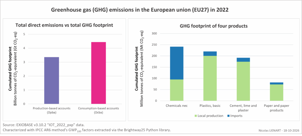
Our approach was to estimate the footprint of both the imported and the locally produced goods within a region of interest. It gives an idea of the hotspot sectors in a given region. In fact, we have estimated the footprint of each of the 200 product categories available in EXIOBASE for both France and the European Union (EU27). Note that the EU27 is not an EXIOBASE region per se, it is an aggregation of member countries we can make from the data. Furthermore, our code can be adapted to any other region (or group) as long as it is available among the 44 regions currently provided by EXIOBASE.

Recent versions of EXIOBASE (3.10.x) do not provide characterized flows. This means that they keep track of the emitted substances, like greenhouse gases (GHGs), as separate flows. We have implemented the characterization of GHGs to obtain the GWP100 results, which is the typical climate change indicator used to account for all major GHGs as a single flow, typically expressed as a unit mass of CO₂ equivalent (e.g., kg CO₂-eq). You may be interested to check the code if you also need to characterize your EXIOBASE results.

Note that in our sector/products analysis, we don’t subtract exports from the results, and it should not be confused with “apparent consumption”. As a consequence, summing all product scores doesn’t result in the total footprint. Doing this would de facto induce double counting of any products entering the value chain of another product within the same region. But don’t panic, we also provide some code at the bottom of the notebook to calculate the region’s consumption footprint and its direct emissions, which this time, doesn’t double count impacts.

Overall, we tried to use default functions of the Pymrio library as much as possible. It was developed by the team behind EXIOBASE and provides an approachable way to manipulate EXIOBASE and alternative EEMRIO via Python.

Overview of bio-based pathway: an interactive online graph database

After identifying the main hotspots among petrochemicals in France and the European Union (EU27), we mapped their bio-based alternatives to produce a graph database of pathways.

By going through an extensive review of the literature we could identify alternative bio-based production routes of the top 50 hotspot petrochemicals (including plastic polymers) in the EU27. There, we have also documented the key building blocks (or platform molecules, intermediates) and the associated production processes. The latter were characterized in terms of their technological and economic maturity, through a simplified technological readiness level (TRL) framework.

We systematically specified the associated literature references. About one hundred bibliographic entries can be found both in the description panel of the online interactive map (Kumu platform) and in the article’s supplementary materials.

Mapping products to ecoinvent geography

A consumption mix based on trade data (BACI)

If you are already familiar with the ecoinvent LCA database you know that many products are split into different “geographies”, which basically relates to where the production or consumption takes place. The inherent variability in the environmental impacts due to regional differences is important to consider in LCA. Changes can happen due to inconsistent standards and regulations, varying feedstocks, waste treatment, transport distances, electric power mix, … Thus, we need to pick the most representative process (or “dataset”) geography (i.e., location/region in ecoinvent’s terms) in the LCA database. This is particularly challenging when we are not so clear about the whole value chain, which is often the case.

Ecoinvent provides some market representative datasets (“market for …”) and according to the official documentation “a market activity represents the consumption mix of a product for a given region, accounting for the trade between the producer and consumer […]”. Said differently “market = consumption mix = production mix + imports – exports, taking transport and losses into account”. However, our analysis revealed that this is not often the case in the database, at least when it comes to petrochemicals. Indeed, during this study we found that these so-called market activities were overwhelmingly more representative of a “production mix” rather than a “consumption mix”, thus remaining limited to what is produced by a region, not to what is consumed inside the regional market.

In our study, we didn’t want to randomly pick datasets to estimate the footprints of the production + imports of chemicals in the EU. This is even more challenging as the granularity of ecoinvent geographies has increased in the succeeding versions of the database. Often, previously available aggregated geographies (e.g., Europe, Rest of the World, Global, etc.) were not kept in recent versions. This increases the difficulty of selecting the right geography.

Let me illustrate this with the case of methanol. In ecoinvent 3.12, the “market for methanol” dataset is available for many geographies: Qatar (QA); Russia (RU); Canada (CA); United States of America (US); Iran (IR); Oman (OM); Rest of the World (RoW); Saudi Arabia (SA); China (CN); Trinidad and Tobago (TT); South America (UN-SAMERICA); Europe without Russia (RER w/o RU). One may think that the last, i.e. “Europe without Russia”, sounds like the most appropriate dataset for our EU27 analysis. However, this one is only representative of the methanol produced within Europe, although most of the methanol passing through Europe is actually imported, as of 2022. This is not self-evident, and we used Eurostat PRODCOM database to estimate the production and imported quantities of products. But PRODCOM data doesn’t distinguish the different origins of products …

To go around this limitation, we have used another database called BACI provided by the CEPII. In essence, it is a reconciled version of the UN’s Comtrade database, tracking trade flows between nations, but without data gaps or inconsistencies (the final balance closes contrary to Comtrade). The great thing about BACI is that trade data is also available in metric tonnes. Mass unit makes much more sense than US dollars when it comes to approximating environmental impacts, both being connected to the physical world.

BACI has a country-level geographical coverage of trade data for around 5,000 products, classified using the 6-digit Harmonized System (HS) scheme. It was necessary to match PRODCOM products to BACI’s HS 2022 codes. To simplify the process and favour reproducibility, we made a Python notebook to perform automatic matching. It builds on top of the official correspondence between PRODCOM and the Combined Nomenclature (CN) provided by the EU, thanks to the CN being compliant with the HS system. Given an input CSV file containing PRODCOM codes, it gives the corresponding HS codes. There were mostly one-to-one matches, with only a few one-to-many which required intervention to pick the most relevant, yet in those few cases it was straightforward.

Once products were matched with an HS22 code, we used BACI data to determine which countries or regions supply the EU27 imports and quantify the share for each selected product. For reproducibility and reuse, we provide another Python notebook containing the code to process the data. It lists all the countries providing each product to the selected region (e.g., the EU27) and calculates their relative market share (in physical quantity).

To estimate the “Europe without Russia” production share, our code automatically conducts suppliers’ aggregation at continental Europe level, excluding all the EU27 member states. Then, the estimated share of each product was subsequently combined with the local production share calculated from PRODCOM, thus yielding the effective share of production originating from Europe which can be mapped to ecoinvent’s “Europe without Russia” region.

Estimating the end of life GHG emissions of petrochemicals

In this study, we wanted to estimate the carbon footprint of major petrochemicals in France (and the EU) to see which of these should be addressed with bio-based substitution.

When we compare ecoinvent products footprints we typically only look at raw materials’ production, and in the case of market activities, we also have the supply footprint (i.e., delivery to the first consumer). By doing this, we omit what happens next during use and disposal of the products. If we want a clear picture of the products’ total footprint, we need to account for that part as well. We call this kind of LCA “cradle-to-grave”, in opposition to “cradle-to-gate” for an assessment which stops at the producer’s or consumer’s gate.

In the context of the SCREEN-LCA demonstration, we neglected the use phase impacts, which are complex to define in the case of bulk chemicals. They intervene in a wide range of downstream products and applications with varying implications. Moreover, the goal of the study was to find substitutes, and thus it should not affect the use phase, especially in the case of drop-in molecules¹.

However, the end of life is a different story. If we switch from fossil ethylene to bio-based ethylene, the end-of-life emissions can be substantially different². So, how can we estimate these GHG emissions in the case of petrochemicals? That seemed as challenging as estimating use-phase emissions at first sight, but we found a way around the complexity.

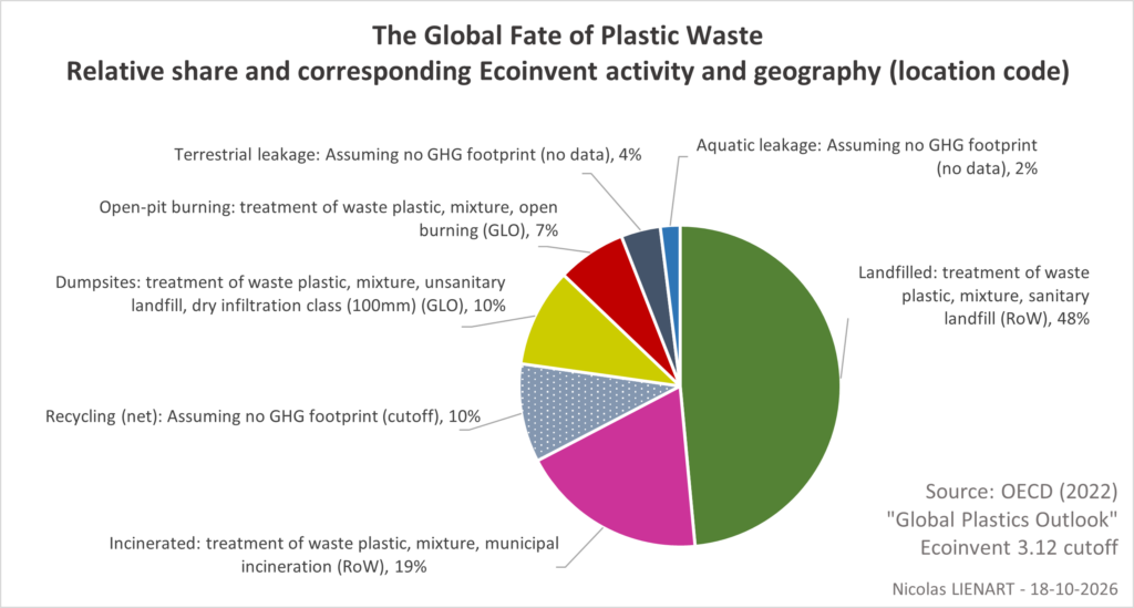
The most prominent petrochemicals produced and imported in the EU are largely related to the plastic industry (e.g., ethylene, propylene, styrene, …). We simplified the issue by considering that the end of life scenario of such chemicals would be best represented by those of plastics. Yet, plastics themselves are diverse, used in variety of contexts, and there are many ways to deal with the waste. Fate depends on polymer type, possible mixing and contamination, and collection method (if it is indeed collected). And since waste flows around the world, use and disposal can happen anywhere. Our solution was to use 2019 global plastic end-of-life statistics from the OECD “Global Plastics Outlook” report. In this study, we assumed acceptable to simplify petrochemical end-of-life by not distinguishing polymer types and uses.

Then we simply mapped the different fates to a generic plastic waste treatment dataset available in the ecoinvent database. Impacts from recycling were excluded as out of the scope. Finally, we did not consider any GHG impacts of the losses to the environment either (e.g., oceans), this time due to lack of corresponding LCA datasets.

An unusual bar chart

At last, I wanted to highlight one outcome which took us some time. It pertains to the presentation of results.

To present our intermediate hotspot results, we have produced a custom figure capable of conveying multiple information at once. This kind of unusual diagram is called a “marimekko” chart.

We took inspiration from the IPCC report which depicted the total footprint of countries by showing both population size and average citizen footprint at the same time (link to this specific figure, see panel c).

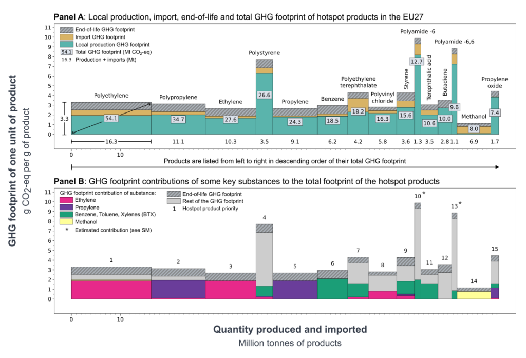
Similarly, we present the product quantity on one other (x-axis) and the unit footprint on the other (y-axis). Each bar’s area is calculated by multiplying the quantity and unit footprint, estimating the total GHG footprint. In addition, we added an extra layer of information by decomposing the footprint. In panel A, we show the share between imports, local production and end-of-life impacts. Below, panel B shows the contribution of a small set of typical building blocks (e.g., ethylene, BTX). This highlights their influence on many petrochemicals and they appear as good candidates for substitution.

All of the code to produce the data, the recursive function which we developed to determine the upstream of the set of substances, along with the code to generate the figure itself are all available in the Git repository.

Footnotes

1. A drop-in molecule is identical to the molecule they replace. For example, bio-based ethylene should behave the same as the current fossil-derived version when it is used in plastics production. This implies that the final product will have similar properties as if it were fossil-based, and thus, not affecting its use or disposal. In our study, we have focused mostly on drop-ins, the exception being PLA and PHAs polymers, which are bio-based alternatives to common polymers like PET. Here, we have neglected the use in our analysis due to the complexity. Therefore, the results should be read as cradle-to-gate + end of life. ↩︎
2. Bio-based products have one determining advantage compared to their fossil counterparts. It has to do with the origin of the carbon. For the reader not familiar with biogenic carbon accounting, one biomass-derived carbon atom (biogenic) can have a substantially different contribution to climate change than one fossil carbon atom. We can consider that it was recently captured from the atmosphere, specifically as CO₂, during biomass growth through the photosynthetic process. Some methods will count this as a negative CO₂ emission (intake = withdrawal = reduced global warming) and count positively every re-emission of carbon as CO₂ as positive, the net can remain negative, sequestrated in the product for a certain amount of time. Other more frequently used methods will just consider that biogenic CO₂ emissions have simply no impact because we are just temporarily “borrowing” CO₂ from the atmosphere. They may however still consider the carbon sequestrated in products (or elsewhere) as never emitted back provided a (very) long lifetime (e.g., landfilled, construction wood, …) but this is debated. ↩︎